8 minutes
Aircraft Simulation in 6 equations
Introduction
Recently, I got into my hands the book Aircraft Control and Simulation written by Stevens and Lewis, this book showcases the theory and design of the main control systems of an aircraft. To test the application of said methods, it is necessary to use a simulator to be able to see the aircraft behaviour after incorporating said controllers.
One obvious choice is to download and use an existing simulator, but as the book already covers the main principles behind simulator design, one will be created and implemented in MATLAB, giving myself full access and understanding of the simulator.
Flat Earth approximation
First of all, because this simulator will be used to test the implementation of control systems in shor- and mid-altitude flights, the Earth will be treated as flat. This is due to the fact that, since the aircraft operates within a relatively small region, the curvature of the Earth has a negligible effect on both flight dynamics and control laws.
To better understand this approximation, one can think of a “flat Earth” as mathematically equivalent to considering an Earth with an infinite radius, where any curvature becomes negligible within the operational area. Given that the Earth’s actual radius is approximately 6,371 km and that typical flight altitudes stay below 20 km, the local surface can be approximated as flat without introducing significant errors. Obviously, this assumption is only valid for short flights (on the order of 50 km or less), but that range is more than sufficient for testing an aircraft’s flight control systems.
The two principal advantages of this approach are, first, that a Cartesian coordinate system (in this case NED, which will be explained later) can be used, and second, that gravity can be treated as a constant vector always pointing in the same direction. These benefits simplify the implementation of the kinematic and dynamic equations.
Reference frames
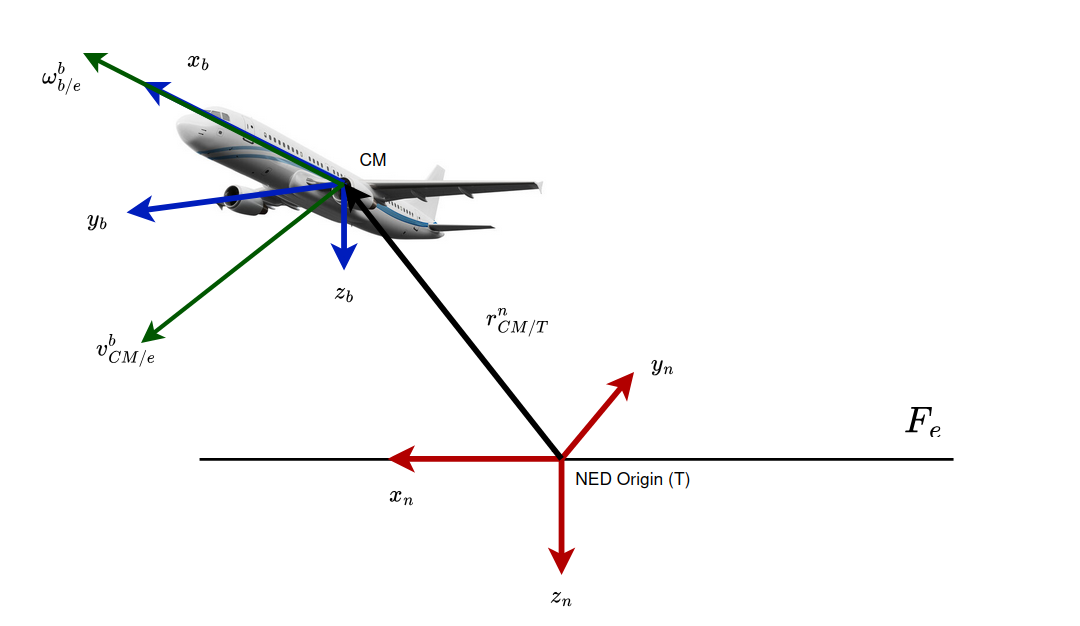
For navigation, the North-East-Down (NED) Cartesian coordinate system will be used. The name is pretty self-explanatory: the X-axis points to the North, the Y-axis points to the East, and the Z-axis points toward the center of the Earth. It is also worth noting that the XY plane (often referred to as the inertial plane or $F_e$) will serve as the reference for calculating the aircraft’s velocities.
On the other hand, the aircraft’s body-fixed moving reference frame is used to define forces, moments, and control inputs. This frame is attached to the aircraft’s center of mass and moves with it. The X-axis points toward the nose of the plane, the Y-axis points to the right wing, and the Z-axis points downward, perpendicular to the aircraft’s wings, as shown in the figure.
6 DOF equations
From the figure, we can see the vectors $\mathbf{v}_{CM/e}^b$ and $\boldsymbol{\omega}_{b/e}^b$. The first represents the velocity of the aircraft’s center of mass (CM) relative to the inertial frame, while the second represents the aircraft’s angular velocity relative to the inertial frame. Note that both vectors are expressed (or “resolved”) in the body frame $b$, meaning that each component of the equations is written in terms of the aircraft’s own axes.
Why are these vectors important?
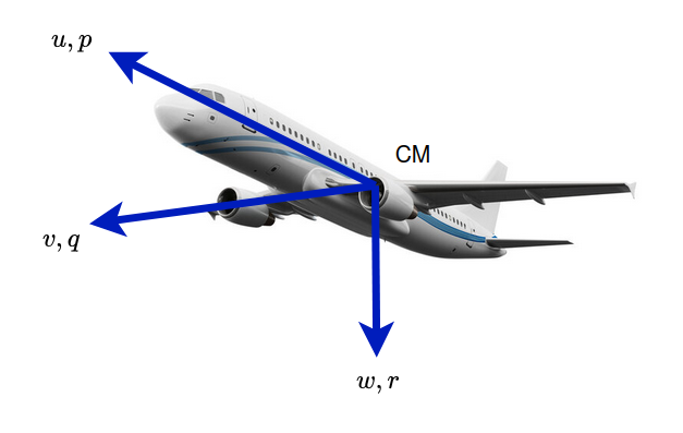
Each of these vectors has three components. Specifically, $\mathbf{v}_{CM/e}^b = [u,\,v,\,w]^T$ captures the velocity along the body-frame’s $X$, $Y$, and $Z$ axes, while $\boldsymbol{\omega}_{b/e}^b = [p,\,q,\,r]^T$ contains the angular rates. Together, these six components (three linear and three angular) describe the aircraft’s motion. Integrating the velocity components yields instantaneous position, and integrating the angular rates yields orientation over time. To derive these vector quantities, one typically applies Newton’s second law.
Translational equation
This equation gives the derivative of the velocity (acceleration) of the body frame in the three principal components. Meaning that it describes how the aircraft speed and direction change over time. The three components of the equations account for:
$$ \dot{v}_{CM/e}^b = \frac{1}{m} F^b + C_{b/m} g^n - (\omega_{b/e}^b \times v_{CM/e}^b) $$- This term reflects the acceleration generated by external forces such as aerodynamic lift and drag, engine thrust, and any other forces acting on the aircraft. In body coordinates, these forces are collected in a vector $F_{A,T}$ which, when divided by the mass, gives the corresponding acceleration in the x,y, and z directions of the aircraft’s body frame.
- This product represents the gravity vector transformed from the inertial frame to the body frame. $g^n$ represents the gravity vector in the inertial frame while $C_{b/n}$ is the rotation matrix that transforms the vector from the inertal frame to the body frame.
I have only included the transformation matrix for reference, but really the first and second columns are neglected as gravity is only acting on the downwards direction. This means that the whole expression boils down to:
$$ C_{b/m} \cdot \mathbf{g}^m = \begin{bmatrix} -g \sin\theta \\ g \sin\phi \cos\theta \\ g \cos\phi \cos\theta \end{bmatrix} $$- This vector product is the Coriolis term, which accounts for the fact that velocity is measured in a rotating frame, ie this acceleration is due to the fact that the aircraft’s body frame is rotating.
By splitting the above vector equation into components along the body axes ((x,,y,,z)), one obtains the following system of non-linear equations:
$$ \begin{aligned} \dot{u} &= \frac{1}{m} F_{x b} - g \sin \theta - w \cdot q + v \cdot r \\ \dot{v} &= \frac{1}{m} F_{y b} + g \sin \phi \cos \theta - u \cdot r + w \cdot p \\ \dot{w} &= \frac{1}{m} F_{z b} + g \cos \phi \cos \theta - v \cdot p + u \cdot q \end{aligned} $$Rotational equation
Just as before, now we are calculating the components of the angular acceleration expressed in the body frame.
$$ \dot{\omega}_{b/e}^b = \mathbf{J_b}^{-1} \left[ \mathbf{M} - \left( \omega_{b/e}^b \times \left( \mathbf{J_b} \omega_{b/e}^b \right) \right) \right] $$The first term accounts for the external moments acting on each of the rotating axis of the aircraft $M=[L,M,N]$ multiplied by the inverse of the moment of inertia matrix. Remember that the moment on inertia, just as mass, expresses a resistance to a change in angular velocity.
The aircraft has three main components of this moments, one for each axis. But we also have the products of inertia, which accounts for the fact that there is coupling between the different axis of the rigid body, meaning that a rotation in one axis creates a rotation in the other one. Assuming that the aircraft is symmetric around the X-axis and the mass is evenly distributed (no fuel movement), some of the terms are null.
$$ \mathbf{J} = \begin{bmatrix} J_{xx} & J_{xy} & J_{xz} \\ J_{yx} & J_{yy} & J_{yz} \\ J_{zx} & J_{zy} & J_{zz} \end{bmatrix} \quad \xrightarrow{\text{Symmetry}} \quad \begin{bmatrix} J_{xx} & 0 & J_{xz} \\ 0 & J_{yy} & 0 \\ J_{zx} & 0 & J_{zz} \end{bmatrix} $$The second term will not be explained in great detail, but it accounts for the gyroscopic effects and coupling between the different axis. Once again, these equations may be expressed as a system of non-linear equations:
$$ \dot{p} = \frac{J_{xz}(J_x - J_y + J_z)pq - \left[J_z(J_z - J_y) + J_{xz}^2\right]qr + J_zL + J_{xz}N}{J_xJ_z - J_{xz}^2} $$$$ \dot{q} = \frac{(J_z - J_x)rp - J_{xz}(p^2 - r^2) + M}{J_y} $$$$ \dot{r} = \frac{-J_{xz}(J_x - J_y + J_z)qr + \left[J_x(J_x - J_y) + J_{xz}^2\right]pq + J_{xz}L + J_xN}{J_xJ_z - J_{xz}^2} $$Combining this three equations and the previous translational ones, one ends up with a system of 6 degrees of freedom which fully describes the dynamics of an aircraft. But we still have something missing, and that is how to define the orientation of the aircraft with respect to the inertial plane?, this is important to determine the aircraft’s attitude.
Euler Angles
To determine the aircraft’s attitude, we use Euler angles, a set of three angles that describe the orientation of the body-frame relative to the fixed coordinate system. We have already used them to determine the direction cosine matrix (DCM) from the inertial frame to the body frame, and that is the main use of these kind of matrices, to determine the vector orientation in one frame to another.
- Roll (ϕ): rotation about the aircraft’s longitudinal (x) axis.
- Pitch (θ): rotation about the aircraft’s lateral (y) axis.
- Yaw (ψ): rotation about the aircraft’s vertical (z) axis.
Now, to get the euler angles from the simulated aircraft (the orientation of the aircraft with respect to the fixed frame), one can transform the body angular rates $(p,q,r)$ from the body frame to obtain the euler rates $(\dot{\phi}, \dot{\theta}, \dot{\psi})$ by simply constructing the DCM from the body to the fixed frame. This procedure involves a series of rotations to aling both the body frame with the inertial frame:
- Yaw rotation $\psi$ about the inertial Z axis
- Pitch rotation θ about the lateral Y′ axis (already rotated by ψ):
- Roll rotation (ϕ) about the aircraft’s longitudinal X′′ axis (rotated by ψ and θ):
When multiplying this matrices in order, one ends up with the final DCM that aids in obtaining the rates for the euler angles.
$$ \mathbf{C}_{I \rightarrow B} = R_x(\phi)\,R_y(\theta)\,R_z(\psi) $$$$ [\dot{\phi}, \dot{\theta}, \dot{\psi}]' = \mathbf{C}_{I \rightarrow B} [p,q,r] $$