9 minutes
Control inputs and coefficients for RCAM model
In our last post, we explored the various forces and moments acting on our model aircraft, tracing how they drive the kinematic equations introduced in the very post. However, while we covered where and how these forces are applied, we have yet to discuss the specific coefficients used to calculate them. In this post, we will dive deeper into quantifying these forces and moments, with a particular focus on how the aircraft’s state variables and control surfaces come into play. As we need to discus the coefficients for a specific aircraft, we’ll use the Research Civil Aircraft Model (RCAM) model, which serves as a baseline to engineers to test and compare different control stategies for civil aircraft usage.
Control inputs
In this scenario, we will only consider the main control surfaces of an aircraft and the thrust of the motors, that means that we will not consider flaps or other (not as important) control inputs. With that in mind, lets examine the main control surfaces of an aircraft:
Ailerons ($\delta_a$) are the small hinged sections located near the wingtips. When one aileron is deflected upward and the other downward, they create differential lift between the left and right wings. This imbalance in lift causes the aircraft to roll, allowing it to bank and turn.
Elevators ($\delta_t$) are control surfaces attached to the horizontal stabilizer (tailplane) at the rear of the aircraft. By moving up or down, they change the pitch angle of the nose, controlling the aircraft’s climb or descent. Deflecting the elevator upward forces the tail down and the nose up, while moving it downward has the opposite effect.
Finally, the rudder ($\delta_r$) is a vertical control surface attached to the fin (vertical stabilizer). It pivots left or right to yaw the aircraft around its vertical axis. The rudder is especially important during takeoff, landing, and crosswind conditions to maintain directional control and coordinate turns when used alongside the ailerons.
Now that we have defined the main control surfaces, we can define our input vector which will control the settings for the angle of the control surfaces and throttle setting. It is important to define this variables beforehand as they will affect the value of the aerodynamic coefficients, so they will aid in the control of the aircraft. It should be noted that each of the control surfaces have the own limits, slew rates and dynamics that shall be included in the simulation, but this will analysed in the future.
$$ u = \begin{bmatrix} \delta_a \\ \delta_e \\ \delta_r \\ \delta_{TH_1} \\ \delta_{TH_2} \end{bmatrix} $$Aerodynamic coefficients in the wind frame
In this section, we will examine the functions to determine the coefficients for the lift, drag and cross-wind forces. First, we will separate the lift coefficient into the wing/body lift coefficient ($C_{Lwb}$) and then the tail component lift coefficient ($C_{Lt}$). Finally, we will calculate the total coefficients for drag and cross-wind.
Wing/body lift coefficient
This coefficient is given by a piecewise function of the angle of attack $\alpha$. The first part of the function defines linearly the value of the coefficient from $\alpha_{L=0}$ which is the angle at which the lift is zero until 14.5 degrees. Then, the coefficient is approximated using a 3rd degree polynomial (the values for the constants can be found in the implementation).
$$ C_{Lwb} = \begin{cases} n (\alpha - \alpha_{L=0}), & \text{if } \alpha \leq 14.5 \frac{\pi}{180} \\[6pt] a_3 \alpha^3 + a_2 \alpha^2 + a_1 \alpha + a_0, & \text{otherwise} \end{cases} $$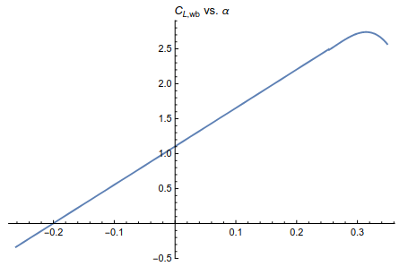
From the figure, we can see that the lift coefficient starts at zero for $\alpha_{L=0}$ and climbs linearly until 14.5 degrees, then we arrive at the point for which the lift is maximum at arround 18 degrees, which is known as the critial angle of attack or stall angle of attack. This value is critical as going beyond this angle leads to a stall condition in which the lift drops dratically.
Tail lift coefficient
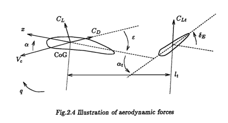
$$ C_{Lt} = \frac{S_t}{S} \cdot 3.1 \alpha_t $$Above is the expression for the lift coefficient for the tail unit, which is entirely dependent on the angle of attack (AoA) of the tail unit ($\alpha_t$). This angle of attack is different to the angle of attack of the aircraft due to the influence of the elevator deflection $\delta_e$ and due to the downwash angle ($\varepsilon$), which represents the local change in airflow direction due to the main wing, meaning that the main wing affects the airflow of the tail unit.
$$ \alpha_t = \alpha - \varepsilon + \delta_E + 1.3 \frac{q l_t}{V_a} $$As said before, the AoA of the tail unit differes from the AoA of the wings due to the to the downwash angle, elevator deflection and dynamic pitch response. The key idea behind this last term is that when the airplane pitches, the tail does not simply see the free-stream flow coming straight on rather, it moves through the air in an arc. That circular motion creates an additional “local” flow component at the tail, effectively changing its angle of attack relative to the incoming flow. This component is modeled using the pitch rate ($q$), the distance between the center of gravity (CoG) and tail unit $l_t$ and the magnitude of the relative velocity $V_a$.
For the equations presented, we are still missing the expression for the downwash angle. It can be calculated using the difference between the $\alpha$ and \alpha_{L=0} due to the fact that when $\alpha=\alpha_{L=0}$, the lift is zero and the flow of the wing do not interferes with the flow of the tail unit, meaning that the downwash angle is null.
$$ \varepsilon = \frac{d\varepsilon}{d\alpha} \cdot (\alpha - \alpha_{L=0}) = 0.25 \cdot (\alpha - \alpha_{L=0}) $$Drag and cross-wind coefficients
The expressions for these two coefficients are much more easy to calculate as the first one is a function of $C_{Lwb}$ and the second one depends on the rudder deflection $\delta_r$ and sideslip angle $\beta$.
$$ C_D = 0.13 + 0.07 \left( C_{Lwb} - 0.45 \right)^2 $$$$ C_Y = -1.6 \beta + 0.24 \delta_r $$Final expression for the forces in the body frame
As stated in the previous blog post, once the force coefficients have been correctly calculated, we can calculate the expressions for the forces in the wind frame just using the dynamic pressure and the wing surface of the aircraft. Then, to transfer the forces from the wind frame to the body frame, just multiply the force vector by the corresponding DCM and then we have the input for the translational equation of motion.
$$ F_a^w= \begin{bmatrix} -D \\ Y \\ -L \end{bmatrix} = \begin{bmatrix} -C_D \cdot q \cdot S \\ C_Y \cdot q \cdot S \\ -C_L \cdot q \cdot S \end{bmatrix} $$$$ F_a^b = C_{w/b}^T \cdot F_a^w $$Moment coefficients in the body frame
Computing the moment coefficients follows a procedure similar to that for aerodynamic force coefficients. However, it’s important to note that while these coefficients are expressed in the body frame, they are derived not at the aircraft’s center of gravity (CoG) but at its aerodynamic center (AC). By definition, the AC is the point at which aerodynamic moments remain constant regardless of the angle of attack. Consequently, after obtaining the moment coefficients at the AC, you must transfer them to the CoG before applying them in the rotational equations of motion.
Moment coefficients
As we can see from the expression bellow, the coefficients can be expressed as the states of a system, which in this case is dependent on the angular rates and the control surface deflections. This system will be analysed at another post in which we will develop control laws for the different control inputs.
$$ \begin{bmatrix} C_l \\ C_m \\ C_n \end{bmatrix} = \begin{bmatrix} -1.4 \beta \\ -0.59 - 3.1 \frac{S_t l_t}{S l} (\alpha - \varepsilon) \\ (1 - \alpha \frac{180}{15\pi}) \beta \end{bmatrix} + \begin{bmatrix} -11 & 0 & 5 \\ 0 & -4.03 \frac{S_t}{S} \frac{l_t}{l} & 0 \\ 1.7 & 0 & -11.5 \end{bmatrix} \begin{bmatrix} p \\ q \\ r \end{bmatrix} + \begin{bmatrix} -0.6 & 0 & 0.22 \\ 0 & -3.1 \frac{S_t l_t}{S l} & 0 \\ 0 & 0 & -0.63 \end{bmatrix} \begin{bmatrix} \delta_A \\ \delta_E \\ \delta_R \end{bmatrix} $$Aerodynamic moments and transfer
$$ M_{AC}^b= \begin{bmatrix} L \\ M \\ N \end{bmatrix} = \begin{bmatrix} C_l \cdot q \cdot S \cdot b\\ C_m \cdot q \cdot S \cdot \overline{c}\\ C_n \cdot q \cdot S \cdot b \end{bmatrix} $$Above is the expression for obtaining the moment vector arround the AC of the aircraft, but as previosly stated, we need to perform a moment transfer from AC to CoG so that the force vector can be the input of the rotational equation, which is obviosly centered arround CoG. For this moment transfer, we need the vector of displacement from AC to CoG ($\Delta$) which can be found in the RCAM document.
$$ M_{AC}^b=M_{AC}^b + F_a^b \times \Delta $$Engine Model
Once we have covered all the coefficients of the aerodynamic forces and moments, we have covered almost all control inputs of our models. However we still need to model the two engines of the aircraft and their corresponding control inputs.
At a first glance, it might seem like a good idea to just add a new force acting on the X-axis of the body, as this is the axis in which the engines are pointing. But due to the fact that the motors are not mounted exactly centered at the X-axis of the plane, they in fact also introduce a torque moment.
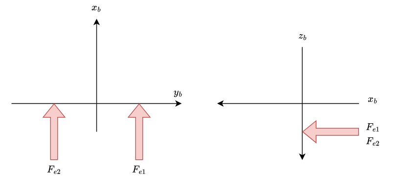
We can model an engine $i$ by simply constructing the force vector which acts on the X-axis and then add engine 1 and 2 to the translational equation. We also need to compute the moment that the motor is generating by mutliplying the position vector $r_{apt}$ (which acts as the moment arm as it describes the point of aplication w.r.t COG) by the force applied by said motor.
$$ F_{ei}^b= \begin{bmatrix} \delta_{THi} \cdot m \cdot g \\ 0 \\ 0 \end{bmatrix} $$$$ M_{ei}^b= r_{apt} \times F_{ei}^b \text{ where } r_{apti} = \begin{bmatrix} X_{apti} \\ Y_{apti} \\ Z_{apti} \end{bmatrix} $$Ending
This is the final post required before starting to program our simulator. In the next one, we will see how we can implement it in MATLAB as a single function so that it can be interpreted as a non-linear system. Also, maybe in the next month or so I will make a more detailed post regarding the aerodynamic forces and moments acting on an aircraft, becuase I have made a lot of simplifications in this post and the last one.