6 minutes
Aerodynamic forces and moments for simulation
In the previous post, we presented the equations of motion for a six-degree-of-freedom (6DOF) system, highlighting how an aircraft’s position and orientation change over time due to the forces and moments acting on the aircraft frame. In this post, we will introduce the aerodynamic forces and moments acting on the aircraft and how they can be modelled.
Stability and wind axis
Lets imagine a fixed model aircraft in a wind tunnel, in which the aircraft is not moving but there is wind from the tunnel (what we call relative wind) which is not centered with the aircraft. To describe the orientation of the wind relative to the aircraft, we use two angles called angle of attack $(\alpha)$ and angle of sideslip $(\beta)$.
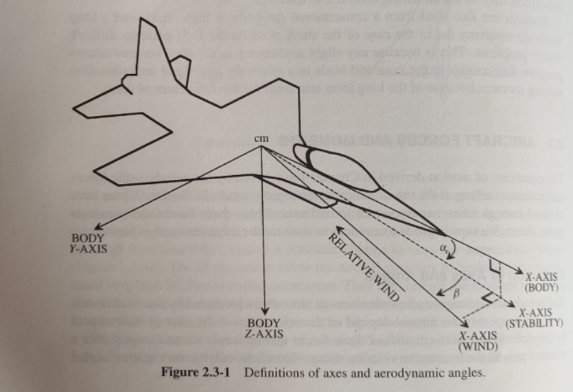
First, we perform a left-hand rotation around $y^b$ (the Y axis of the body frame) until the relative wind vector is in the XY plane. This rotation gives the angle of attack which is positive when the relative wind comes from below the nose of the aircraft. When performing this transformation, one ends up in the stability axis, whose DCM is found below.
$$ C_{s/b} = \begin{bmatrix} \cos \alpha & 0 & \sin \alpha \\[6pt] 0 & 1 & 0 \\[6pt] -\sin \alpha & 0 & \cos \alpha \end{bmatrix} $$Then, one can perform a left-hand rotation around $z^s$ (the Z axis of the stability frame) to align the relative wind vector to the X axis of the new frame, which is known as the wind frame. This angle is known as angle of sideslip and the DCM to go from the stability frame to the wind frame is found below.
$$ C_{w/s} = \begin{bmatrix} \cos \beta & \sin \beta & 0\\ -\sin \beta & \cos \beta & 0\\ 0 & 0 & 1 \end{bmatrix} $$Now that we have the DCM from the body to stability frame, and stability frame to wind frame, we can also compute the DCM from body to wind frame:
$$ C_{w/s} C_{s/b} = C_{w/b} = \begin{bmatrix} \cos \alpha \cos \beta & \sin \beta & \sin \alpha \cos \beta \\ -\cos \alpha \sin \beta & \cos \beta & \sin \alpha \sin \beta \\ -\sin \alpha & 0 & \cos \alpha \end{bmatrix} $$Relative velocity
Now, instead of a fixed aircraft, we consider a moving aircraft in the atmosfere, in this case we consider can consider a vector opposite of the relative wind, which we call relative velocity. This vector captures the aircraft’s velocity as experienced by the surrounding air. Considering that there is no wind in the simulator, the module of the relative velocity will be the same as the module of the velocity of the aircraft, ie $v_{CM/e}^b$. However, the angle of attack and sideslip will be dependent on the aircraft’s orientation (if for example the nose is pointing up or down). This is to illustrate that the angles of the wind axis and the module can be calculated using the components of $v_{CM/e}^b$ and that $v_{rel}$ is aligned with the X axis of the wind axis.
$$ V_{\text{rel}}^b = \begin{bmatrix} U \\ V \\ W \end{bmatrix}= C_{b/w} V_{\text{rel}}^w= C_{b/w} \begin{bmatrix} V_T \\ 0 \\ 0 \end{bmatrix}= \begin{bmatrix} V_T \cos \alpha \cos \beta \\ V_T \sin \beta \\ V_T \sin \alpha \cos \beta \end{bmatrix} $$Then, the module, angle of attack and sideslip can be calculated as:
$$ \| v_{rel} \|_2 = V_t = \sqrt{u^2 + v^2 + w^2} $$$$ \alpha = \arctan \left( \frac{w}{u} \right) $$$$ \beta = \sin^{-1} \left( \frac{V}{V_T} \right) $$Atmosferic model
As we will see in the next section, forces that act on the airplane are dependent on dynamic pressure or $q$ which is essentially the “push” the airflow exerts on an object when the object is moving. Mathematically, it’s given by:
$$ q = \frac{1}{2} \rho V_T^2 $$Where $V_T$ is the norm of the relative velocity and $\rho$ is the density of the air. However, air density is dependent on the altitude, that is why we need an atmosferic model to determine the air density at any given altitude.
Many simulators use the U.S. Standard Atmosphere 1976 model as it is valid up to 82 km, but it will require to input all the formulas in MATLAB or use interpolators for the tables. Instead, I am just going to use the International Standart Atmosphere block, which can be used up to 32 km (typical passegenger jets fly at 11 km over sea level).
Aerodynamic forces
Three primary forces are used to describe how an aircraft responds to the airflow. First, the Lift force acts on the Z-axis of the wind frame and counters the airplane’s weight, increasing with speed and angle of attack to help the aircraft stay aloft. On the other hand, Drag opposes the direction of the relative wind (on $x^w$) and slows the aircraft, arising from friction. Finally, Cross-wind is oriented with $y^w$ (vector going out of the screen) and captures any sideways “push” caused by crosswinds or fuselage and tail interactions. These three forces together define the aerodynamic resistance and directional behavior of the aircraft.
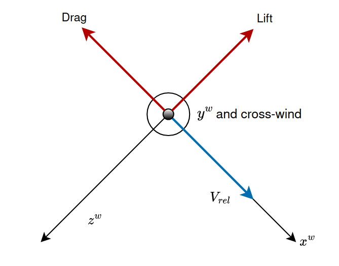
As can be seen in the figure, the forces are expressed alongside the axis of the wind frame, so finally we can get the numerical expressions for the three forces using the dimensionless coefficients for each force, the dynamic pressure and the wing-span of the aircraft:
$$ F_a^w= \begin{bmatrix} -D \\ Y \\ -L \end{bmatrix} = \begin{bmatrix} -C_D \cdot q \cdot S \\ C_Y \cdot q \cdot S \\ -C_L \cdot q \cdot S \end{bmatrix} $$The terms $C_L$, $C_D$ and $C_Y$ are the lift coefficient, drag coefficient, and side-force coefficient, respectively. Each of these coefficients is typically derived from either wind tunnel tests or computational simulations and takes into account parameters such as the airplane’s geometry, angle of attack, sideslip angle and other factors. By using these coefficients along with the dynamic pressure term, we can predict how large each aerodynamic force will be under various flight conditions without having to solve any complex fluid equations. Manufacturers normally present these coefficients in lookup tables or curve fitted polynomials to predict the values for different angles of attack, airspeed and other conditions. This will be covered in more detail in the near future when we model a specific aircraft.
Finally, as the forces are expressed in the wind frame, we need to transform them into the body frame to use the 6DOF model. However, this transformation is pretty easy as we can just use a transformation matrix. This is due to the fact that, to obtain the DCM from body to wind frame, we can just transpose the matrix to get the DCM from wind to body ($C_{b/w}=C_{w/b}^T$).
$$ F_a^b = C_{w/b}^T \cdot F_a^w $$Aerodynamic moments
The analysis for the moments is pretty much the same as for the forces, meaning that to calculate each one of the three moments we shall use the specific coefficient, the dynamic pressure and the surface of the wings. Also remeber that, as moment is equal to a force times a moment arm, the expressions of the moments require to be multiplied by the wingspan ($b$) or mean aerodynamic chord ($\overline{c}$).
$$ M= \begin{bmatrix} L \\ M \\ N \end{bmatrix} = \begin{bmatrix} C_L \cdot q \cdot S \cdot b\\ C_M \cdot q \cdot S \cdot \overline{c}\\ C_N \cdot q \cdot S \cdot b \end{bmatrix} $$With these expressions, we have succesfully developed the expressions for the aerodynamic forces and moments that act on an aircraft. In the next blog post, we will examine how to calculate the coefficients for the forces and moments using a real aircraft model.